DECISION TREES

Decision Trees

Motivation:

Classification techniques for analysts have majorly been Logistic Regression, Decision Trees and SVM. Due to some of the following limitations of Logistic Regression, Decision Trees prove to be very useful:

1. Doesn’t perform well when the feature space is too large
2. Doesn’t handle large number of variables/features well
3. Linear decision boundary layers

Tree

What are decision trees?

Decision trees are a powerful prediction method and extremely popular. They are popular because the final model is so easy to understand by practitioners and domain experts alike. The final decision tree can explain exactly why a specific prediction was made, making it very attractive for operational use

Representation

Given below is an example of a decision tree classifying whether a day is suitable for playing tennis .

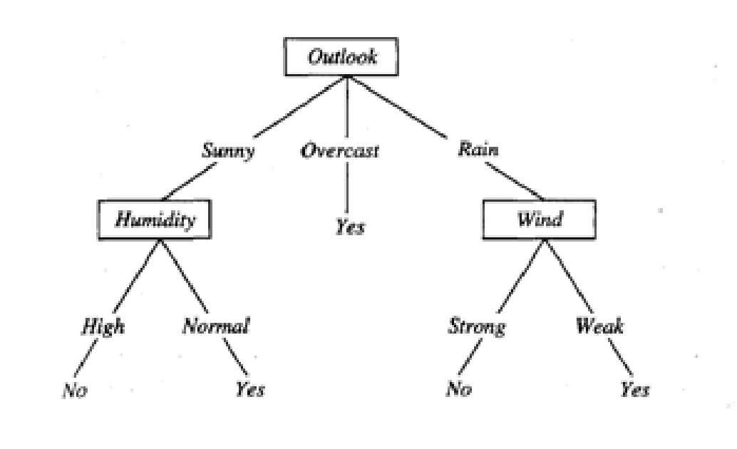
A decision tree consist of three main parts - root nodes , leaf nodes , branches .It starts with a single node called “root node ” which then branches into “child nodes” . At each node , a specific attribute is tested and the training data is classified accordingly.

In the above example , the root node tests the attribute “Outlook” and splits into 3 branches according to the 3 values taken by the attribute - “Sunny” , “Overcast ”and “Rain” .

Regression vs Classification

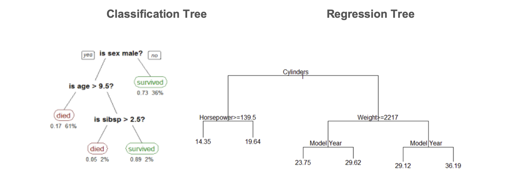
Classification trees are used when the target variable is categorical in nature whereas Regression trees are used when the target variable is continuous or numerical in nature

In case of linear regression , a single formula is used for prediction in the entire training data set. But if the number of features are more , they can interact in non-linear ways and modelling a single formula becomes difficult .Hence regression trees are used.

A regression tree is built through a process known as binary recursive partitioning, in which the dataset in partitioned into smaller regions until we obtain data sets where we can fit simpler models.

Classification trees works in the same manner, only the predictor variables are categorical in nature.

Building a Model:

Choosing a split criteria to to start forming child nodes is the first step in a building our decision trees. There are many index or measures available to test the homogeneity of a sample after a split, some of the popular ones are mentioned below

Popular cost functions :

1. Information gain :

Information gain measures the reduction in entropy caused by classifying the training data on the basis of an attribute. Higher the information gain ,better is the attribute in classifying the data.

Mathematically,

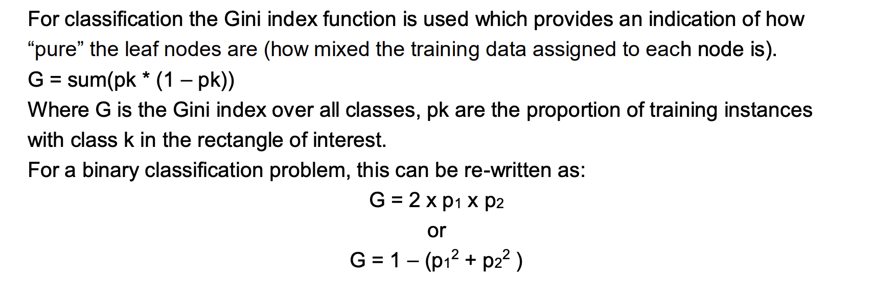
2. Gini Index :

3. Chi - square test :

Chi-square is another test used to determine the statistical significance between the parent node and the child-nodes after the split.

Evaluating the performance of Decision trees :

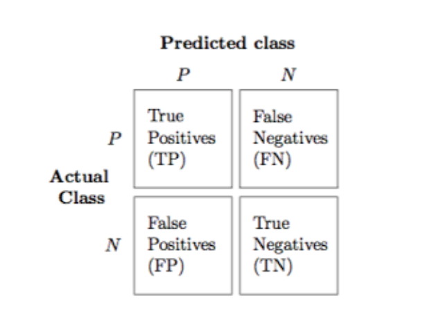
Confusion Matrix : The performance of the decision tree over the test data set can be summarised in a confusion matrix.
The each training example will fall into one of the four categories -

1. True Positives (TP) : All positive instances correctly classified
2. False Positives (FP) : All negative instances incorrectly classified as positive.
3. False Negatives (FN) : All positive instances incorrectly classified as negative
4. True Negatives (TN) : All negative instances correctly classified

Accuracy can be calculated from the table as the ratio of correct predictions to total predictions .

However, calculating accuracy alone is not very reliable if the number of datasets belong to each class are very different .

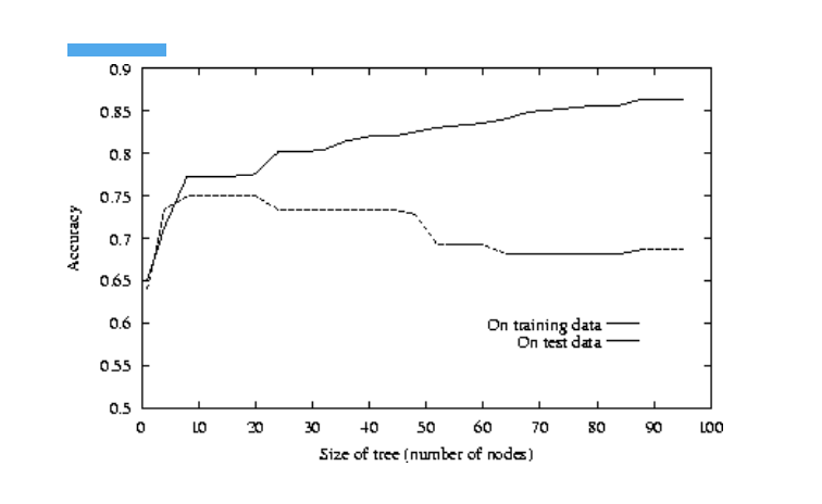
Decision trees are prone to overfitting . If they are grown too deep , they lose generalisation capability .

Tree pruning :

Pruning is a general technique to avoid overfitting by elimination the branches of the tree that provide little power to classify data .

Some of the popular pruning strategies are :

1. Cost Complexity pruning : A series of pruned trees are generated by removing a sub-tree and replacing it with a leaf node . The optimally pruned tree among these is the one with the least cross-validated error .
2. Reduced error pruning : In this method , a sub-tree is replaced by a leaf-node and if the prediction accuracy is not affected significantly , the changes are kept .

Random forests :

As discussed earlier , when working with large sets of data decision trees often run into the problem of overfitting. Hence, an ensemble learning technique called Random Forests is used.

Ensemble Learning refers to using multiple learning multiple learning algorithms to make better predictive models. Some of the common ensemble learning types is bagging, boosting, bayesian parameter average etc.

As the name suggests random “forest” is a combination of large number of decision “trees”. A random forest grows multiple trees.

To classify a new object based on attributes, each tree gives a classification which is then aggregated into one result .The forest chooses the classification by the number of votes from all the trees and in case of regression, it takes the average of outputs by different trees.

Random forests are considered more popular than single decision tree due to the fact that they can minimise overfitting without bringing in much error of bias .

Despite being more accurate , the random forest algorithms are computationally expensive and hard to implement .

Implementation

We’ll break down our implementation on the banknote case study into the following for steps:

1. Data Exploring and Pre-processing
2. Data Splitting
3. Building Model
4. Making Predictions

Data Exploring and Pre-processing:

This is how a snapshot of our data looks like:

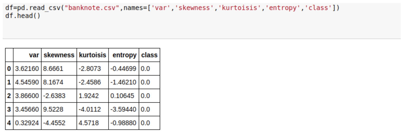
To give a brief background of the data and the column headers:

Data was extracted from images that were taken from genuine and forged banknote-like specimens. For digitization, an industrial camera usually used for print inspection was used. The final images have 400 x 400 pixels. Due to the object lens and distance to the investigated object grayscale pictures with a resolution of about 660 dpi were gained. Wavelet Transform tool were used to extract features from images.

The variables and their respective denotion goes as follows:

• Var: variance of Wavelet Transformed image (continuous)
• Skewness: skewness of Wavelet Transformed image (continuous)
• Kurtosis: kurtosis of Wavelet Transformed image (continuous)
• Entropy: Entropy of image(continuous)
• Class: DIscrete variable accounting for the class in which the banknote lies

The is taken from the UCI Repository:
http://archive.ics.uci.edu/ml/datasets/banknote+authentication
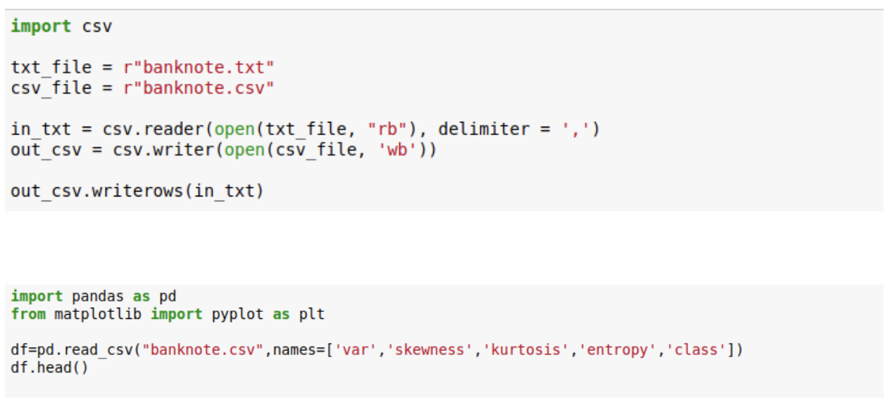
The data has no null values and any other cleaning are also not needed, only column headers need to be added and converting the txt file to csv with a comma delimiter is needed. The implementation for the same is:

For data exploration we start with multivariate analysis to get an idea of how the decision boundary might look like

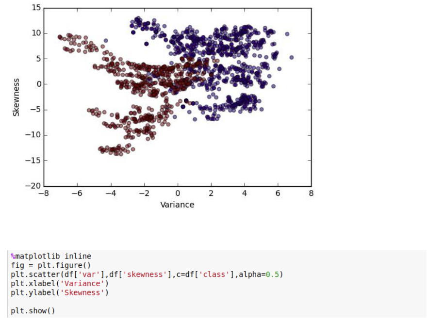
A little idea about the decision boundary can be gathered from the above visualization, where the Red dots represent class 0 and blue represent class 1.

Building the Model:

We’ll be using two splitting techniques and then compare the better model. In each case we would need to split the data into train and test set, done as below: (As of now we have limited the maximum tree depth, we would discuss the reasoning behind later)

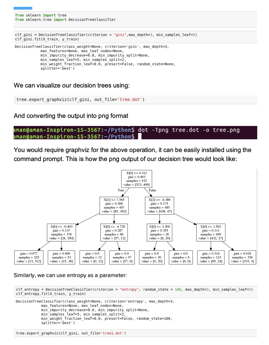
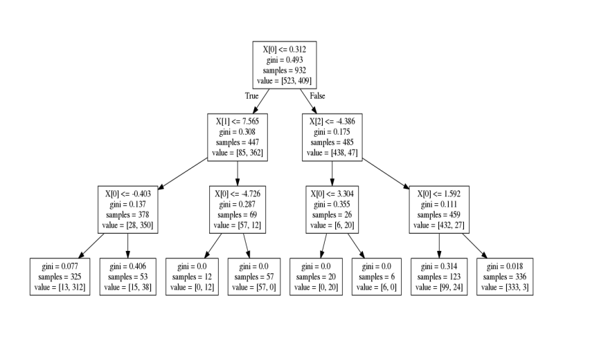
Performance of the Model

Sklearn has a module for accuracy metrics, we would fit both the models and check their accuracy:

Random Forests

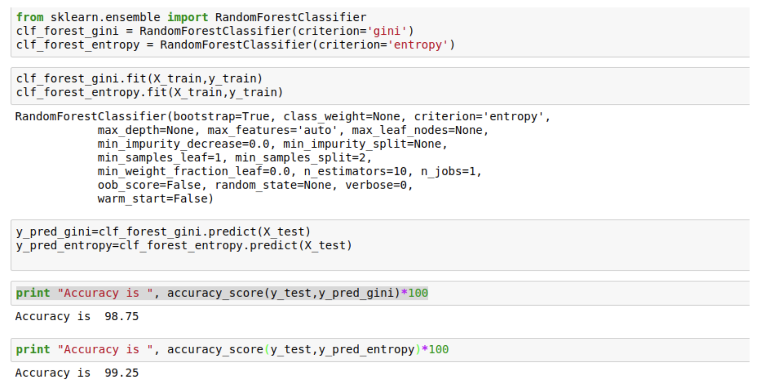
As you can see the accuracy of both the models have improved significantly.

A new dimension to the study of Decision Trees comes after learning about bagging and boosting. These topics have been covered in advanced modules